Building a crypto spillover pipeline

The question needed a measurement system

For my 2026 Master's thesis, I wanted to understand whether economies with more open capital accounts were more exposed to cryptocurrency volatility. When crypto markets became turbulent, did their equity and foreign-exchange markets show stronger Bitcoin-associated connectedness?

The study covered 2019 to 2025. It began with 89 configured economies; data-quality rules retained 86 in at least one market channel. I could construct usable spillover measures for 77 equity markets and 81 FX markets, starting with Bitcoin prices recorded every minute.

I split the question into two stages: construct a daily measure of connectedness for each market, then examine how that measure varied with crypto stress and country characteristics.

For anyone building analytical pipelines, the useful parts are the decisions around those models. I'll walk through how I handled missing observations and mismatched calendars, then explain why the resulting metric complicated the conclusion I wanted to draw from it.

Answering that question required building two things: a reliable international market-data pipeline and a rolling statistical measurement system.

The inputs disagreed about time and meaning

Input	Original frequency	Main complication
Bitcoin and Ethereum, Binance	One minute, 24/7	Exchange gaps and UTC day boundaries
National equity indices	Daily	Local holidays, incomplete histories, mixed providers
FX rates	Daily	Opposite quotation conventions and nearly fixed rates
VIX, dollar index, S&P 500, Brent	Daily	Missing dates differ from local markets
Openness and exchange-rate regime	Annual	Country-year joins and unavailable recent vintages
GDP per capita and private credit/GDP	Annual	Reduced to country averages for 2019 to 2023

Yahoo Finance covered many markets. Others required manually downloaded Investing.com or official-source files. Three-character country IDs connected those sources to institutional data; ticker symbols alone could not identify a country consistently.

The panel builder starts from the union of observed equity and FX country-date pairs. Market returns join on both fields. Bitcoin variance and global controls join by date; annual institutions join by country and year. Crypto restrictions come from dated episodes.

The column called dxy illustrates why those source definitions matter: it contains FRED's broad trade-weighted dollar index, DTWEXBGS, rather than the ICE DXY index. The panel builder makes the joins explicit, but understanding them still requires following each input back to its source.

Keeping acquisition and analysis inspectable

The system uses files as intermediate artifacts. Bronze Parquets hold downloaded or parsed inputs, silver Parquets hold cleaned market series, and gold Parquets hold analytical variables and model outputs.

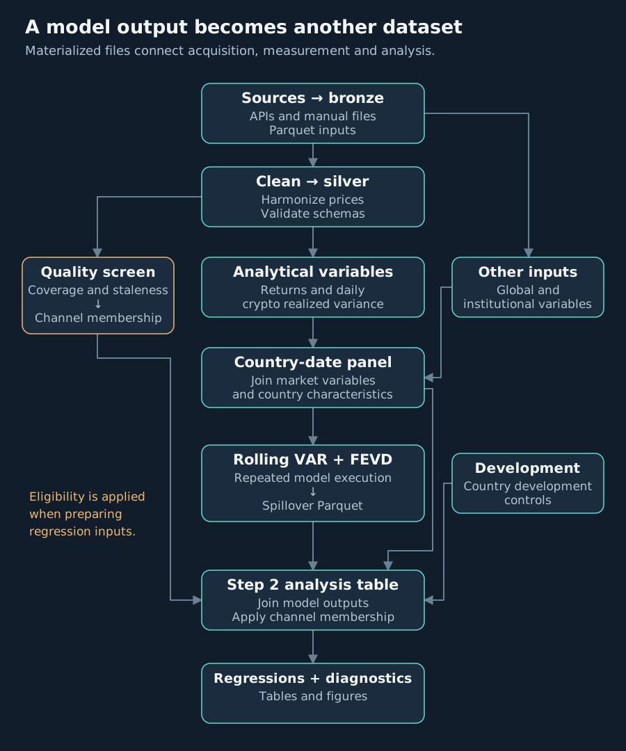
The quality screen is a separate branch. The rolling engine computes measures from the broader panel; membership is applied when preparing the regression inputs. That separation lets me inspect a market's data and model output without admitting it into the estimation sample.

The Makefile records dependencies between many of these artifacts. For example, the spillover file depends on its builder, the rolling implementation, schemas, and the input panel. Changing the estimator can rebuild that output without downloading market prices again.

Materializing the stages also makes investigation easier. An implausible share can be traced through the input panel to cleaned prices and the original source. I can inspect those files before rerunning an expensive analytical stage.

The environment is recorded in uv.lock, and GitHub Actions installs it before running pytest. Integration tests that require locally built data skip when those files are absent. Reproducing the empirical results therefore requires the data artifacts as well as the code and environment.

Data cleaning needed explicit rules

Missing observations stay missing

Forward-filling a price invents an observation:

Observed:       100 -> missing -> 105
Forward-filled: 100 -> 100     -> 105
                       ^
                 artificial zero return

That zero can distort the distribution of returns and any volatility estimate built from it. Its effect depends on the statistic: inserting a zero does not change the sum of squared returns in this tiny example, but it changes the observation count and the apparent sequence of daily movements.

The pipeline computes returns between consecutive observed closes. A return after a holiday therefore spans the closure and is attributed to the reopening date, preserving the interval the prices actually describe.

This policy is specific to prices. Annual openness values are carried across daily observations, and the latest available 2023 value carries into 2024 and 2025. Filling a slowly updated institutional attribute and inventing a market price are different analytical decisions.

Normalize FX quotes at the cleaning boundary

The Yahoo XXXUSD=X series used here quote dollars per unit of local currency. Manual FX inputs use local currency per dollar. The cleaning code inverts the Yahoo values so the silver layer consistently means local currency per USD: an increase means depreciation.

Reciprocating a rate reverses its log-return sign, so squaring the return removes that sign difference in Step 1. The convention still matters for interpreting rates and calculating depreciation-based crisis flags elsewhere. Fixing it once saves every downstream consumer from remembering which provider used which convention.

Flag probable glitches without deleting every large move

A large price change may be a feed error or a real crisis. The retrospective heuristic in clean_markets.py drops an observation only when its absolute log return exceeds 0.5 and the move from that price to the price two observations later exceeds 0.5 in the opposite direction.

That is a large reversal check, not a requirement that the price return exactly to its previous level. It preserves large moves that persist, but it can still misclassify a genuine sharp reversal. Because it looks ahead, it belongs to retrospective cleaning and would need reconsideration in a live system.

Make invalid rows fail at a boundary

The silver FX contract in src/quality/schemas.py checks the fields downstream code relies on:

FX_CLEAN = DataFrameSchema(
    {
        "date": Column(pa.DateTime, nullable=False),
        "country_id": Column(str, Check.str_length(3, 3), nullable=False),
        "ticker": Column(str, nullable=True),
        "fx_rate_vs_usd": Column(float, Check.gt(0), nullable=False),
        "source": Column(str, Check.isin(["yahoo", "investing"]), nullable=False),
    },
    unique=["country_id", "date"],
    strict=True,
    coerce=True,
)

The required price must be positive, country-date keys must be unique, and unexpected columns fail validation. The country check enforces length; it does not validate membership in the ISO country list.

An unresolved exchange-rate regime gets a -1 sentinel, and the panel builder refuses to consume it. The error names the countries still needing classification, so I can resolve the missing information before it becomes a regression variable.

Decide market eligibility before inspecting coefficients

A series can cover the whole study period and still offer little information for volatility measurement if its price hardly ever changes.

The quality screen measures coverage against the study window's Monday-to-Friday business-day count, and staleness as the fraction of consecutive observed prices that are identical. The thresholds live in config/sample_rule.yaml: coverage of at least 80%, with staleness capped at 20% for equity and 40% for FX. Managed currencies can legitimately remain unchanged more often than equity indices, which motivates a separate FX threshold.

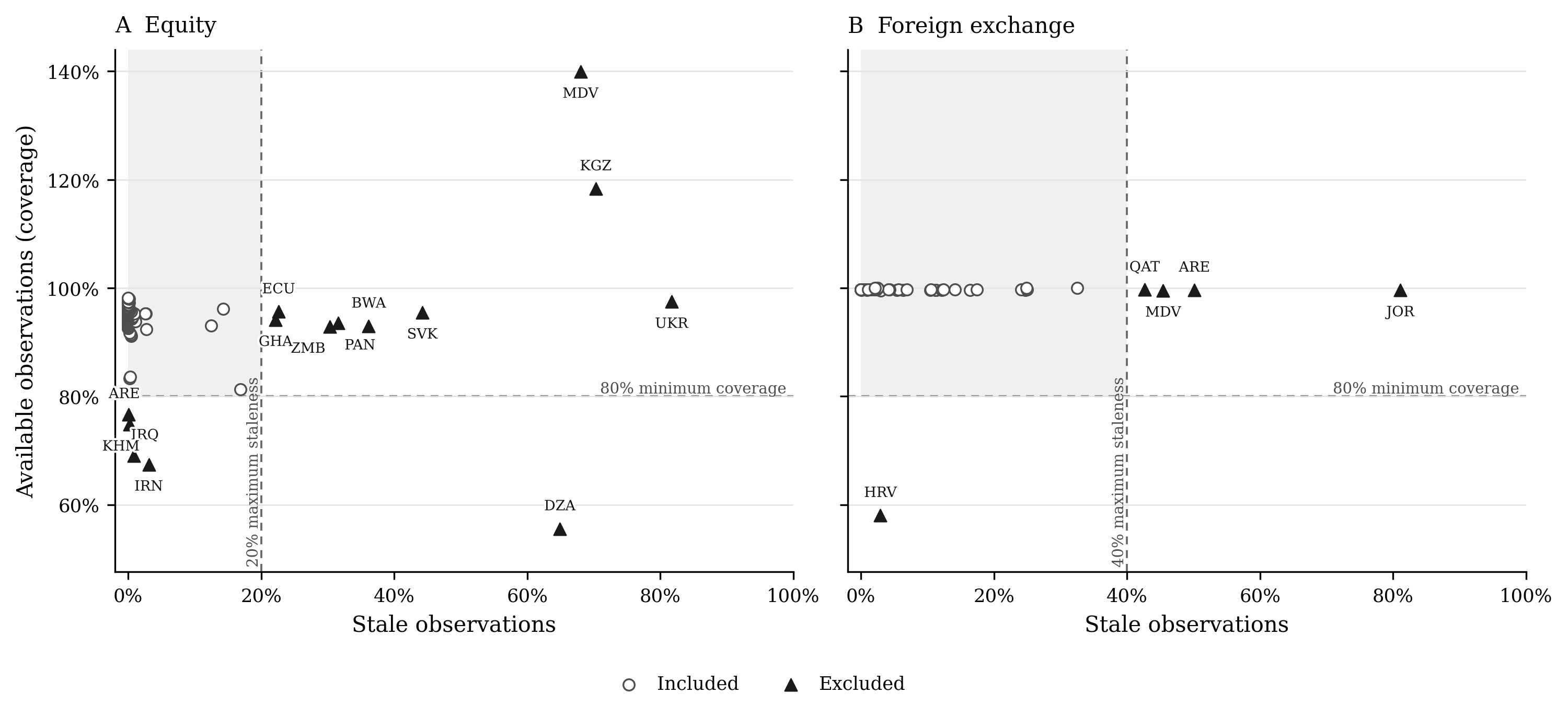
Coverage uses a generic weekday denominator, not each exchange's holiday calendar. Sources containing weekend observations can exceed 100%; the chart preserves that limitation.

Each country-channel decision gets a pass/fail value and an exclusion reason. The rule consumes price-quality metrics, with no regression coefficients as inputs. This makes a sample change something to explain and reproduce.

Of 89 configured economies, 86 qualified somewhere. Seventy-eight equity series passed the quality rule; the thesis records Venezuela's subsequent numerical estimation failure, leaving 77. FX contributed 81 estimable series.

Those counts describe where the measure is available. A regression also needs its explanatory variables: the baseline models with full controls use 71 equity and 75 FX countries. Reporting the count at each stage makes the losses visible. These counts are documented in thesis section 3.2.3 and Appendix A.5.

Turning paired volatility series into a daily share

I needed a measure of how Bitcoin volatility and local-market volatility evolved together, with enough flexibility to change over seven years.

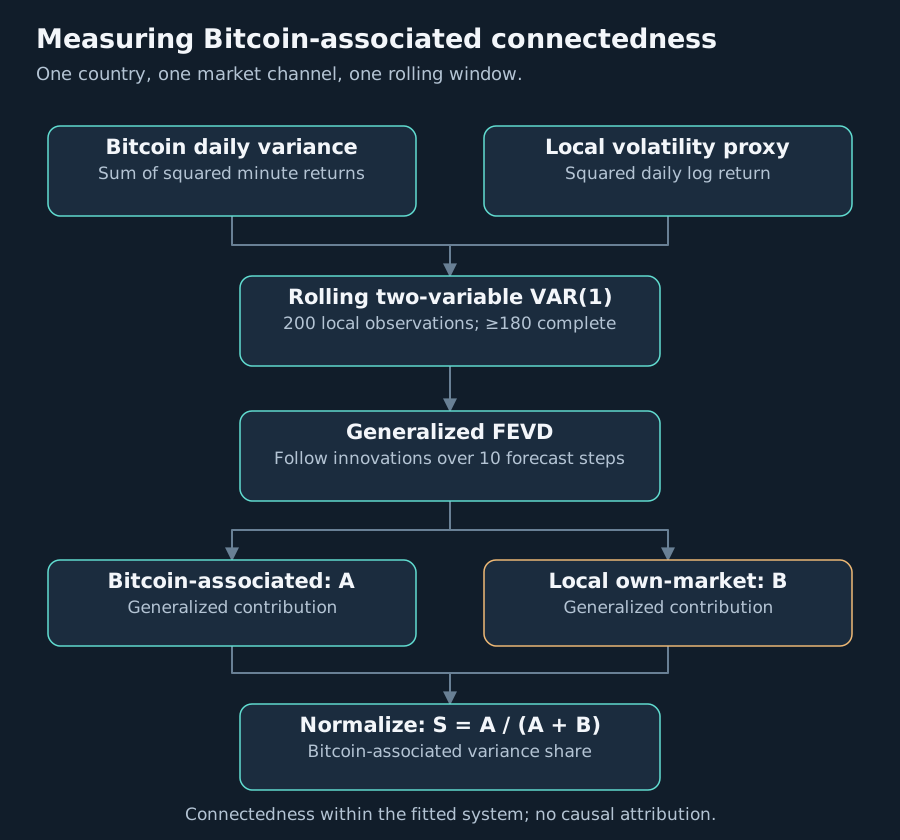
For Bitcoin, the pipeline calculates log returns between observed minute prices, squares them, and sums them by UTC date. This is daily realized variance: large intraday movements contribute more than small ones. Domestic markets usually offer only daily closes, so their proxy is the squared log return between consecutive observations.

These measure movement at different resolutions. Bitcoin's intraday variance can capture movement that disappears by the daily close; the domestic proxy cannot.

Fit the pair on a moving window

I wanted each series' recent history to help explain how the pair evolved. A vector autoregression, or VAR, fits that joint system. In a VAR(1), today's Bitcoin variance is modelled using both series' previous values, and today's local volatility proxy is modelled the same way. Each equation has an intercept and an unexplained innovation: the part its lagged inputs did not predict.

One fit over the whole study would impose constant coefficients. Instead, I refit the pair over a trailing window of 200 local-market observations, requiring at least 180 rows where both inputs exist. Every estimate is dated at the window's end.

This excerpt from src/spillovers/rolling_dy.py follows selection of dates with observed local returns. It is verbatim, with surrounding setup omitted:

    values = trading[["btc", "local"]].to_numpy()
    for i in range(window - 1, len(trading)):
        win = values[i - window + 1 : i + 1]
        synced = win[~np.isnan(win).any(axis=1)]
        if len(synced) < min_obs:
            continue
        out.iloc[i] = _gfevd_share(synced, horizon=horizon, lag=lag)
    return out

The clock is local observations, not 200 calendar days. The forecast horizon is ten steps on that observation grid.

Alignment still has a limit. A Monday equity return may span Friday's close to Monday's close, while its Bitcoin input covers Monday's UTC day. Matching the date fields does not make those intervals identical. This is a daily connectedness design, not precise event-time attribution.

Allocate forecast uncertainty without privileging a variable order

Once the pair is fitted, I need to ask how much uncertainty in the local volatility forecast is associated with innovations on the Bitcoin side of the system.

Forecast-error variance decomposition, or FEVD, follows innovations through the fitted model over a chosen horizon and measures their contributions to forecast uncertainty.

A common decomposition uses Cholesky factorization to make innovations uncorrelated. It requires an ordering: the first variable receives priority in allocating contemporaneous shared variation. Reversing the order can change the answer. I had no defensible reason to give either Bitcoin or the domestic market that priority.

The generalized approach avoids that arbitrary ordering. The implementation computes it from the fitted VAR's moving-average coefficients and residual covariance matrix, then normalizes each target row to sum to one. The reported value is the local row's Bitcoin entry.

Generalized contributions can overlap because innovations are correlated. Row normalization produces a comparable share, but it does not establish separate causal sources. A common global shock can move both inputs. "Bitcoin-associated" therefore means connectedness within this fitted system; it does not mean Bitcoin caused the movement.

The rolling-model tests go beyond checking bounds. They simulate a system with a known directional relationship and compare it with independent series. A function that always returned a plausible number between zero and one would fail that check.

A model output became another dataset

Step 1 writes data/parquet/gold/spillovers.parquet. Its actual layout has one row per country-date and separate channel columns:

date | country_id | spill_equity | spill_fx | window | horizon | var_lag

The schema checks uniqueness, bounded shares, and specification metadata. A missing channel remains null; the builder omits dates where neither channel produces a value.

This is the interface between the stages. The regression layer can consume shares without running a VAR itself, and reporting can read coefficient artifacts without fitting regressions. The model has become a transformation that produces another inspectable dataset.

That boundary also changes what provenance means. For a derived share, the price source alone is insufficient: the window, lag, and forecast horizon help define the observation.

Explaining differences without treating every row as independent

The second stage asks whether the relationship between crypto stress and the Bitcoin-associated share differs with openness.

KAOPEN, the Chinn-Ito index, describes restrictions on cross-border financial transactions. I use its normalized zero-to-one version as a moderator. The term of interest is openness × crypto stress: it allows the stress slope to differ between relatively restricted and relatively open economies.

Conceptually, the pooled regression is:

share ~ openness + crypto stress + openness × crypto stress
        + restrictions + development controls + global controls

The continuous stress variable is the log of a trailing mean of Bitcoin realized variance. Averaging smooths daily spikes, and taking logs compresses the long right tail. Behind the thesis's "21-day" shorthand, panel_prep.py computes a 21-observation mean over distinct dates present in the market panel. It is not an explicit 21-calendar-day window over the full Bitcoin history.

Ordinary independent-error standard errors would ignore two dependencies. Adjacent 200-observation windows reuse 199 observations when the inputs are complete, making successive shares highly related. Countries also share the Bitcoin series and global conditions.

The primary estimator is pooled OLS with Driscoll-Kraay standard errors, which accommodate temporal and cross-country dependence under their assumptions. The implementation allows dependence across up to 200 time lags, capped for short samples, with Bartlett weights that decline for more distant lags.

This changes uncertainty estimates around the fitted coefficients. It cannot remove omitted-variable bias, make the design causal, or propagate all uncertainty from estimating the first-stage shares. Those require separate attention.

The first result was negative

Bitcoin-associated shares varied over time and were strongly skewed to the right:

Country-day share	Equity	FX
Mean	5.79%	2.45%
Median	1.43%	0.84%

The typical observation was much smaller than the mean. Large shares in part of the distribution pulled the average upward.

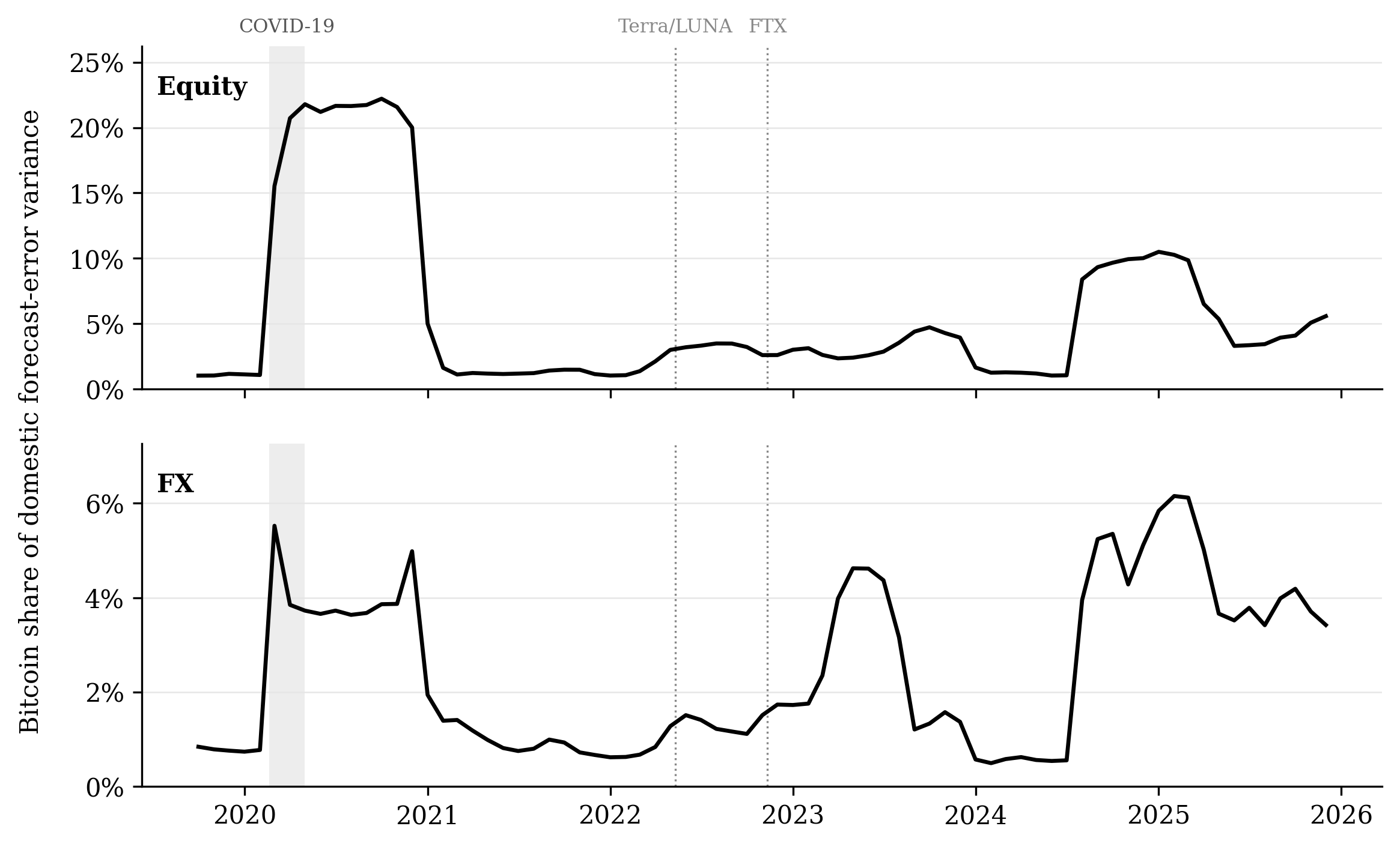
Monthly means pool available country-day shares. The panels use different vertical scales. Event markers provide context; they do not identify causal effects.

I initially expected openness to amplify the stress relationship. In the baseline pooled FX model, the interaction was negative: β = −0.0065, p = .015.

To check sensitivity to the bounded, skewed outcome, I clipped shares at their first and 99th percentiles, then transformed them to log odds, log(S / (1 - S)). This also produced a negative interaction, β = −0.420, p = .006. These are the thesis's reported baseline results.

The negative interaction means the fitted stress slope becomes smaller as openness increases. It does not, by itself, say that the share falls with stress in every open economy. Interpreting it as protection from Bitcoin volatility would require several further assumptions, beginning with what the share measures.

A falling share can hide an unchanged contribution

The bivariate implementation stores a Bitcoin-associated generalized contribution, A, and a local own-market contribution, B. Its normalized share satisfies:

$$S = \frac{A}{A+B}$$

Consider this illustrative example:

Case	Bitcoin contribution A	Local contribution B	Bitcoin share
Initial	2	8	20%
Larger local contribution	2	18	10%

Bitcoin's contribution is unchanged. Its share halves because the denominator grows. A decrease in A could also lower the share; the ratio alone cannot tell us which happened.

This is familiar in other datasets. An error proportion can fall while the number of errors stays constant if total traffic grows. A market share can fall while sales increase. Before assigning a mechanism to a percentage, inspect the quantities it divides.

A + B is the denominator used to normalize the generalized contributions. Because innovations can correlate, it need not equal the local forecast-error variance. The code stores that variance separately as local_var, allowing the diagnostics to examine both quantities.

The component regressions did not show a stable reduction in Bitcoin's unnormalized contribution. Some local-variance diagnostics supported a larger-denominator interpretation under fixed effects, including a separate measure built directly from squared returns. Pooled estimates did not provide the same support. The final thesis's component analysis therefore treats the mechanism as suggestive and estimator-sensitive.

The openness interpretation weakened for another reason. The baseline already included GDP per capita and private credit as controls, but allowing them to also interact with crypto stress made the FX openness interaction statistically indistinguishable from zero.

Controlling for development's average relationship with the outcome had not allowed development to change the stress slope. Once it could, the design could no longer distinguish openness as an independent moderator. That does not establish financial development as the cause; it limits what I can attribute to openness.

Try to break the interpretation

I treated robustness checks as specific ways the conclusion could fail:

Change	Failure mode being investigated
60-observation window, minimum 54 synchronized rows	The 200-observation measure smooths over shorter relationships
Winsorized log-odds outcome	Bounded, skewed shares make conclusions depend on outcome scale
Country and date fixed effects	Pooled differences reflect persistent country traits or shared dates
Ethereum in Step 1	The measure depends on Bitcoin as the transmitting asset; Step 2 retains Bitcoin stress
Drop crisis-flagged countries	Extreme inflation or depreciation dominates the coefficient
Openness interactions with VIX and the broad dollar index	Crypto stress stands in for broader global conditions
Development interactions with crypto stress	Openness stands in for a correlated development characteristic
Broad dollar factor in the first-stage VAR	Bitcoin is allocated variation also associated with dollar conditions
Exclude unstable VAR windows	Numerically explosive fits distort shares or component diagnostics
Keep one euro-area representative	Several country IDs repeatedly weight one underlying currency

The shorter FX windows retained the negative direction but gave weaker evidence. Crisis exclusions and the stability screen did not remove the baseline pattern. Ethereum and the three-variable dollar system were sensitive to the outcome transformation; fixed-effects results also depended on the specification. The thesis's robustness results do not support calling the finding universal.

The euro check exposed a problem that a schema could not catch. In notebook 10, 18 countries share the same euro-dollar FX series; 16 sit at maximum openness. Their country-date keys are unique, yet they repeatedly represent one currency's movements.

Keeping one euro representative reduced the interaction from about −0.0065 to −0.0037, with p around .30. Driscoll-Kraay accounts for dependence in standard errors, but does not reweight the pooled coefficient. A uniqueness constraint can pass while the analytical unit remains questionable.

The stability diagnostic recomputes an unfiltered baseline alongside the filtered models. Comparing both in the same run reduces the risk of attributing a change to the filter when code or samples changed between saved artifacts.

What I would redesign today

Make time and coverage explicit inputs

I would calculate the stress series directly from the complete daily Bitcoin artifact and specify calendar days or observations deliberately. I would also carry minute coverage into the panel, define how incomplete crypto days enter estimation, and examine crypto variance over intervals closer to local close-to-close returns. The current code records coverage but does not use it as a baseline eligibility rule.

Complete the build dependencies

The Makefile captures much of the workflow, but the panel target omits the restriction-episode file it reads, report targets lack input prerequisites, and make all can reach a World Bank fetch through crisis flags. I would make every file read a declared dependency and split external acquisition from local derivation consistently. Then an edited input would invalidate the relevant outputs predictably.

Keep a record of every rolling estimate

The rolling implementation catches fitting exceptions and returns missing output without retaining the reason. Missing values can therefore mean insufficient synchronized data or a failed fit. I would write a companion diagnostic table with country, channel, window boundaries, usable-row count, failure reason, and stability measure. That would make numerical exclusions easier to explain and investigate.

Version the inputs behind a result

The lockfile records software dependencies; it does not freeze downloaded market history. I would add content hashes and a run manifest linking source snapshots, configuration, code commit, and derived artifacts. That would make it easier to tell whether a changed result came from revised data or revised analysis.

Extend the research inputs

One global Binance USDT price does not measure local crypto pricing or flows. Local prices, stablecoin flows, and more detailed policy changes could support better questions about transmission. Richer first-stage systems could include global factors directly. Each extension would change what the measure can represent and would need its own validation.

What I would carry into another project

The most reusable work happened around the model: defining a valid observation, preserving the intervals behind a date, and keeping enough intermediate data to investigate a result.

I would use the same approach for any pipeline that turns repeated model fits into metrics. Give those outputs a schema, record how they were constructed, and inspect the underlying quantities before interpreting a change. In this project, that meant following a negative coefficient back through the share's denominator, competing moderators, and repeated currency series. Each check narrowed the claim I could defend.

Source code and figures · Full Master's thesis